Pavement evaluation
Network screening and project investigation answer different questions
Calculate conditional screening rates, reconcile nested populations and distinguish programme selection from diagnostic accuracy.
Editorial preview · Technical review pending
Network screening identifies questions; investigation develops answers.
Coverage before confidence
The brightest warning on a network dashboard may also be the least corroborated.
FWD benchmarking is used in the context of both network monitoring and rehabilitation investigation. The interpretation depends on the question being asked. (Horak, 2008)
Follow a hundred flags through review
Governing relationship: Flagged = 20/100; retained = 16/20; investigated = 6/16.
Nj: records retained at stage j. Each conditional denominator is the prior stage.
Counts are 100, 20, 16 and 6. All review sets are nested.
The film first plots records, then follows the calculation and plots retention (%). Only 6% of the original set reaches investigation. The conditional 37.5% at the last stage uses a denominator of 16, not 100.
Selection accounting
From network to investigation
Selection rates describe the process, not the probability of failure.
Model, calculations and transcriptEquations, worked steps, source notes and a timed reading guide
Understand the model
A screening funnel follows nested sets. Each stage has its own conditional denominator.
Work through the inputs and equations below, then compare the calculated output with the film. All numerical inputs in this study are synthetic.
Inputs and symbol key
- Nj; Nj−1
- Section counts at the current and preceding review stages.
- pj
- Conditional retention fraction at stage j (dimensionless).
Values used in this film
- Nj: records retained at stage j. Each conditional denominator is the prior stage.
- Counts are 100, 20, 16 and 6. All review sets are nested.
The mathematical relationships
Equation 1
Source and scopeFor each stage, divide the number retained by the preceding-stage count.
Equation 2
Source and scopeThe middle counts cancel because the sets are nested. Multiplying the conditional rates gives the fraction of the original population investigated.
Work through the example
Use the relationships above with consistent units. These substitutions are our worked example, not values quoted from the source.
Flagged fraction
20 / 100 = 0.20
fraction of screened
QA retention
16 / 20 = 0.80
fraction of flagged
Investigation retention
6 / 16 = 0.375
fraction of QA set
Combined fraction
0.20 × 0.80 × 0.375 = 0.06
fraction of original set
Read the output
Only 6% of the original set reaches investigation. The conditional 37.5% at the last stage uses a denominator of 16, not 100.
Check your understanding
Verify set membership, not just decreasing totals. Confirm the six investigated identifiers occur in the sixteen-section QA set and reconcile additions, removals and deferred sections between snapshots.
Assumptions and limits
Selection rates describe the process, not the probability of failure.
Return to the full references and method notes to check the cited edition and its applicability.
Timestamped film transcript 29 short entries · select a time to revisit the film
From network to investigation. Nested synthetic review sets; no predictive classifier.
MATHEMATICS · define the relationship and the meaning of each symbol before calculating.
Nj: records retained at stage j. Each conditional denominator is the prior stage. Counts are 100, 20, 16 and 6. All review sets are nested.
INPUT · records at each stage · read the axis units and the numerical values.
Nested synthetic review sets; no predictive classifier.
Screened: 100 of 100 scheduled records (100.0%). Grey records remain visible.
Flagged: 20 of 100 scheduled records (20.0%). Grey records remain visible.
Retained after QA: 16 of 100 scheduled records (16.0%). Grey records remain visible.
Investigated: 6 of 100 scheduled records (6.0%). Grey records remain visible.
OUTPUT · conditional retention · read the axis units and the numerical values.
Only 6% of the original set reaches investigation. The conditional 37.5% at the last stage uses a denominator of 16, not 100.
CALCULATION · substitute the defined inputs; keep units through each intermediate step.
Flagged fraction: 20 / 100 = 0.20 fraction of screened
QA retention: 16 / 20 = 0.80 fraction of flagged
Investigation retention: 6 / 16 = 0.375 fraction of QA set
Combined fraction: 0.20 × 0.80 × 0.375 = 0.06 fraction of original set
SENSITIVITY · change one declared input · read the axis units and the numerical values.
Investigate 4: 4 % of original 100. Four of the sixteen QA sections proceed.
Investigate 6: 6 % of original 100. Six of the sixteen QA sections proceed.
Investigate 8: 8 % of original 100. Eight of the sixteen QA sections proceed.
Check: Verify set membership, not just decreasing totals. Confirm the six investigated identifiers occur in the sixteen-section QA set and reconcile additions, removals and deferred sections between snapshots.
ONE ROW · The brightest warning on a network dashboard may also be the least corroborated.
PARAMETER MAP · 12000 evaluated cells. The colour limits stay fixed across every row.
Each of the 12,000 cells joins four synthetic deliveries on a route-section key. A source is present unless its declared modular missingness rule removes that row. Count the
present sources and divide by four; the downloadable network exercise below contains the individual deliveries. Use the map to ask where source availability is thin before
attaching a structural interpretation to a screening flag. Height shows coverage only; the route axis is an identifier, not a geographical coordinate.
VALUE LANDSCAPE · Height and colour encode Available-source fraction. This is a graph over the two input axes, not automatically a physical pavement shape.
This computed source fraction is not classifier confidence, probability of failure or a real evidence inventory. Source presence, independence, quality and relevance must be checked separately in a field application.
Selection rates describe the process, not the probability of failure.
Download the timed captions (VTT)
The transcript records the on-screen wording. Formula provenance and interpretation are explained in the source note above.
Write the decision before selecting data
For screening, define the flag and the evidence that merits follow-up. For a project investigation, identify which uncertainty needs to be resolved. Keep the transition from flag to investigation visible in the record.
Follow a flagged section
A synthetic map highlights a section after a survey. The reviewer first checks location and measurement quality, then considers corroborating observations and the investigation brief. The demonstration ends with a question to investigate, not a prescribed treatment.
What belongs in the investigation handover
A network colour is not a design. Avoid presenting a screening result with the precision or authority of a completed project investigation.
Make the handover a question
A screening handover might say: “This synthetic section needs review because the latest measurement differs from its neighbouring sections; position and acceptance evidence have been checked.” It should identify the supporting records and the question that remains.
The investigation brief can then ask what additional evidence would distinguish competing explanations. That step prevents a map flag from becoming a treatment instruction through repetition.
Keep the scope of the decision explicit. Prioritising where to investigate, establishing the cause of distress and selecting a rehabilitation design are different decisions. A team can make useful progress on the first without pretending to have completed the others.
Account for what happens after a flag
Imagine 100 network sections are screened. Twenty are flagged for review, 16 of those have passed the planned data-quality checks, and six have received a project investigation. These are nested populations: the bars should not be added together.
Case review
A flag needs a question attached to it
Which of the original 100 sections has enough evidence for the next decision?
The discriminating check
For each flagged section, inspect location, survey acceptance and the availability of corroborating sources.
Evidence supports the comparison
With usable evidence, state the uncertainty the project investigation should resolve and choose discriminating observations.
Evidence is missing or incompatible
With missing or incompatible sources, make evidence repair the next task; do not rank an unknown as a healthy section.
What you can conclude. Use the four-source exercise below to inspect coverage. Source count is not classifier confidence or probability of failure.
Original worked case. Read the source editions and method notes.
The flagged share is 20 / 100 = 20%. The investigated share of flagged sections is 6 / 20 = 30%. Neither percentage measures pavement severity, and neither specifies a treatment. Four flags still need their quality questions resolved; ten quality-checked flags have not yet reached the investigation stage in this example.
This distinction matters in programme reporting. A map with many reviewed flags may show progress in screening while little project evidence has yet been gathered. Calling all of those sections “investigated” overstates the work and obscures the next resource decision.
A screening handover should state the reason for the flag, the evidence checked and the question that remains. The investigation brief should then identify which uncertainty it is intended to resolve. For example, a locally elevated response may warrant a review of its consistency with other measurements and observations before an intervention is developed.
Horak discusses structural benchmarking in a broader pavement-evaluation context. A relative response can help identify a question; it does not make a network flag equivalent to a completed rehabilitation design. (Horak, 2008)
The practical result is a more honest programme: screening identifies where attention may be useful, quality review establishes whether the records support the concern, and project investigation develops the evidence for a design decision. Each stage has a distinct output and a distinct basis for completion.
Calculation laboratory
What does a six-percent investigation rate tell us?
| Calculation step | Substitution or result | Units and interpretation |
|---|---|---|
| Flagged fraction | 20 / 100 = 0.20 | fraction of screened |
| QA retention | 16 / 20 = 0.80 | fraction of flagged |
| Investigation retention | 6 / 16 = 0.375 | fraction of QA set |
| Combined fraction | 0.20 × 0.80 × 0.375 = 0.06 | fraction of original set |
The product works because the populations are nested and the numerator of one ratio cancels the denominator of the next. It does not assume statistical independence. If QA includes additional sections selected through another route, the cancellation no longer describes this funnel and the register must represent those entrants explicitly.
The final percentage measures programme selection, not diagnostic accuracy. We cannot calculate sensitivity, specificity or a false-negative rate from these counts because the actual condition of the uninvestigated sections is unknown. Labelling the ninety-four remaining sections “sound” would therefore invent evidence. A validation sample drawn from outside the flagged set can help investigate missed cases, with its sampling design recorded.
The sensitivity cases change investigation capacity while holding the prior review sets fixed. They show how many of the original hundred sections reach detailed investigation, not how much risk has been reduced. Project-level questions still require evidence about mechanism, geometry and loading. Keep the selection reason, excluded records and review dates so that a future engineer can distinguish a low-priority decision from a missing or invalid measurement. The network/project distinction is consistent with the investigation framework in TRH12. (Department of Transport, 1997)
Controlled sensitivity experiment
| Controlled case | Calculated output | What changes |
|---|---|---|
| Investigate 4 | 4.000000 % of original 100 | Four of the sixteen QA sections proceed. |
| Investigate 6 | 6.000000 % of original 100 | Six of the sixteen QA sections proceed. |
| Investigate 8 | 8.000000 % of original 100 | Eight of the sixteen QA sections proceed. |
What does a six-percent investigation rate tell us?
Compare the cases on a fixed scale. Select a case to inspect its input change and calculated output.
Reproduce and challenge the result
Verify set membership, not just decreasing totals. Confirm the six investigated identifiers occur in the sixteen-section QA set and reconcile additions, removals and deferred sections between snapshots.
These are original synthetic calculations. The sensitivity cases vary the stated input while retaining the other assumptions; they are not field observations or treatment thresholds. The film’s calculation and sensitivity chapters use the same numerical cases as this table.
Map the gaps before interpreting the flags
Each of the 12,000 cells joins four synthetic deliveries on a route-section key. A source is present unless its declared modular missingness rule removes that row. Count the present sources and divide by four; the downloadable network exercise below contains the individual deliveries. Use the map to ask where source availability is thin before attaching a structural interpretation to a screening flag. Height shows coverage only; the route axis is an identifier, not a geographical coordinate.
Reproduce the experiment. c = (profile present + FWD present + visual present + drainage present)/4. The downloadable table contains 12,000 evaluated cells, with the two input coordinates and output value retained on every row. These are parameter combinations, not that many independent field observations. The equation extends the worked example above; it is original teaching arithmetic, not a new standard or calibrated prediction.
Coverage before confidence
The brightest warning on a network dashboard may also be the least corroborated.
Download every calculated cell (CSV) · Open full-size explorer · Equation source and tests (ZIP)
This computed source fraction is not classifier confidence, probability of failure or a real evidence inventory. Source presence, independence, quality and relevance must be checked separately in a field application.
Four deliveries walk into a join
The real complication is seldom another decimal place. It is four teams describing the same road with four different records. Here is a reproducible rehearsal: 60 routes, 200 equal 100 m sections per route, one lane and one survey month. That makes 12,000 location keys, not 12,000 independent experiments.
The profile source contains a prescribed response 3 + 0.5 sin(section/9) + 0.25 cos(route/7) m/km. The FWD source uses the homogeneous centre-settlement equation w₀ = 2(1 − ν²)P/(πaE) with E = 200 + 60 sin(section/13 + route/5) MPa, 40 kN, 0.15 m radius and ν = 0.35. This second source follows the elastic reference, not a regression from roughness. (FHWA, 2017) (University of Cambridge, 2005)
The visual source varies integer rutting ratings while retaining K = 2,534.1666667 and other contributions totalling 195.069357733. It follows the fully worked VCI example, including the small-degree factor and final nonlinear transform. The drainage source supplies a categorical outlet code (section + route) mod 3; those codes describe three invented inspection states and carry no numerical severity weight. They do not feed a pavement-damage model. (CSRA, 1994)
Each delivery deliberately omits a different repeatable subset of rows. Join on route + lane + chainage + month, preserve empty values and count source availability. The source fraction is the number of present sources divided by four. It is neither confidence nor probability of failure. Joining does not make the surveys contemporaneous in a real project; the common month is an explicit simplification here.
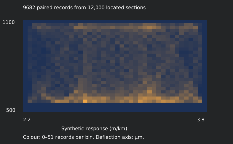
A density plot counts overlapping points instead of painting a solid cloud. The horizontal bins are 0.04 m/km wide and the vertical bins are 20 μm high. Colour reports the count in each bin. This reveals the distribution of the paired inputs without pretending that a dense cluster establishes a causal relationship or a treatment threshold.
Download the joined table, then inspect the separate profile, FWD, visual and drainage deliveries. The count manifest makes dropped or duplicated records detectable. A useful student exercise is to compare the all-four-source subset with the paired profile/FWD subset and explain why their denominators differ.
The dataset is intentionally synthetic. Its regular patterns come from the equations and missingness rules in the generator, not from South African field observations. Before using this workflow on a project, replace those assumptions with the actual survey support, source quality and approved interpretation rules.
References and method notes
- Horak (2008). Benchmarking the structural condition of flexible pavements with deflection bowl parameters. Journal of the South African Institution of Civil Engineering, 50(2), pp. 2–9. Original source (Accessed: 5 September 2026).Relative structural benchmarking with deflection bowls
- Department of Transport (1997). TRH12: Flexible Pavement Rehabilitation Investigation and Design. Draft TRH12, Pretoria: Department of Transport for COLTO. Original source (Accessed: 5 September 2026).Chapter 1: rehabilitation design process; investigation, evaluation, analysis and economic appraisal
- FHWA (2017). Using Falling Weight Deflectometer Data With Mechanistic-Empirical Design and Analysis, Volume III. FHWA-HRT-16-011, Chapter 2. Original source (Accessed: 5 September 2026).Deflection testing guidelines
- University of Cambridge (2005). Engineering Tripos Part IIA: 3D5 Geotechnical Engineering. Examination paper and formula information, 2005. Original source (Accessed: 5 September 2026).Data sheet Sections 3.1 and 3.3, printed pp. 6 and 8: circular-load stress and surface settlement
- CSRA (1994). Draft TRH22: Pavement Management Systems. Pretoria: Department of Transport, 1994. Original source (Accessed: 5 September 2026).Technical Addendum A.3, equations A.3.1–A.3.3 and Table A.3.1, printed pp. 125–126; Section 6.2.2, printed pp. 55–56, for alternative-weight normalisation
Use the source edition and project requirements that apply to your work. Educational examples are not site-specific design advice.